# simulate data
N <- 100000
X <- runif(N, min = 0, max = 20)
u <- rnorm(N, sd = 10)
# population regression
Y <- -2 + 3.5 * X + u
population <- data.frame(X, Y)
# set sample size
n <- 100
# compute the variance of beta_hat_0
H_i <- 1 – mean(X) / mean(X^2) * X
var_b0 <- var(H_i * u) / (n * mean(H_i^2)^2 )
# compute the variance of hat_beta_1
var_b1 <- var( ( X – mean(X) ) * u ) / (100 * var(X)^2)
# print variances to the console
var_b0
#> [1] 4.045066
var_b1
#> [1] 0.03018694
# set repetitions and sample size
n <- 100
reps <- 10000
# initialize the matrix of outcomes
fit <- matrix(ncol = 2, nrow = reps)
# loop sampling and estimation of the coefficients
for (i in 1:reps){
sample <- population[sample(1:N, n), ]
fit[i, ] <- lm(Y ~ X, data = sample)$coefficients
}
# compute variance estimates using outcomes
var(fit[, 1])
#> [1] 4.186832
var(fit[, 2])
#> [1] 0.03096199
# divide plotting area as 1-by-2 array
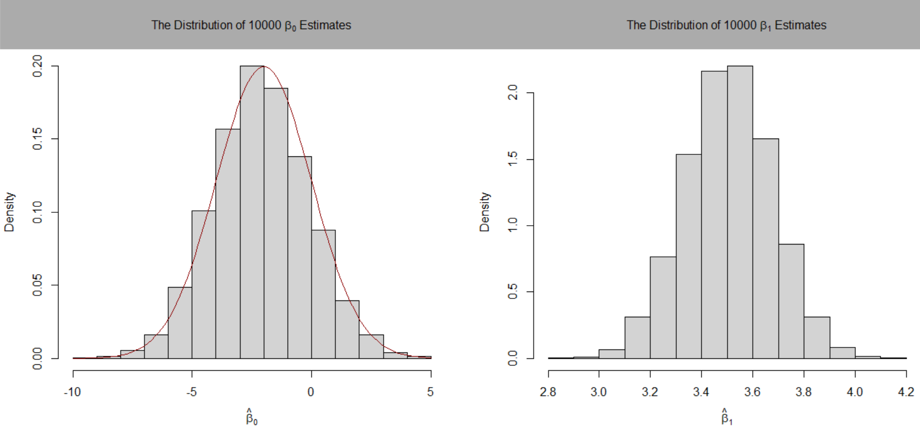
par(mfrow = c(1, 2))
# plot histograms of beta_0 estimates
hist(fit[, 1],
cex.main = 1,
main = bquote(The ~ Distribution ~ of ~ 10000 ~ beta[0] ~ Estimates),
xlab = bquote(hat(beta)[0]),
freq = F)
# add true distribution to plot
curve(dnorm(x,
-2,
sqrt(var_b0)),
add = T,
col = “darkred”)
# plot histograms of beta_hat_1
hist(fit[, 2],
cex.main = 1,
main = bquote(The ~ Distribution ~ of ~ 10000 ~ beta[1] ~ Estimates),
xlab = bquote(hat(beta)[1]),
freq = F)
# add true distribution to plot
curve(dnorm(x,
3.5,
sqrt(var_b1)),
add = T,

