library(AER)
library(stargazer)
data(HMDA)
head(HMDA)
str(HMDA)
HMDA$deny <- as.numeric(HMDA$deny)
str(HMDA)
HMDA$deny <- HMDA$deny -1
str(HMDA)
denymod1 <- lm(deny ~ pirat, data = HMDA)
summary(denymod1)
windows()
# plot the data
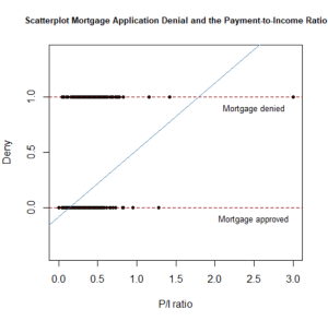
plot(x = HMDA$pirat,
y = HMDA$deny,
main = “Scatterplot Mortgage Application Denial and the Payment-to-Income Ratio”,
xlab = “P/I ratio”,
ylab = “Deny”,
pch = 20,
ylim = c(-0.4, 1.4),
cex.main = 0.8)
# add horizontal dashed lines and text
abline(h = 1, lty = 2, col = “darkred”)
abline(h = 0, lty = 2, col = “darkred”)
text(2.5, 0.9, cex = 0.8, “Mortgage denied”)
text(2.5, -0.1, cex= 0.8, “Mortgage approved”)
abline(denymod1,
lwd = 1.8,
col = “steelblue”)
windows()
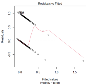
plot(denymod1,1)
windows()
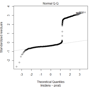
plot(denymod1,2)
# estimate the simple logit model
denylogit <- glm(deny ~ pirat,
family = binomial(link = “logit”),
data = HMDA) #glm是廣義的意思
summary(denylogit)
windows()
# plot data
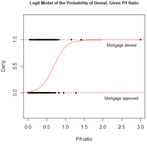
plot(x = HMDA$pirat,
y = HMDA$deny,
main = “Logit Model of the Probability of Denial, Given P/I Ratio”,
xlab = “P/I ratio”,
ylab = “Deny”,
pch = 20,
ylim = c(-0.4, 1.4),
cex.main = 0.85)
# add horizontal dashed lines and text
abline(h = 1, lty = 2, col = “darkred”)
abline(h = 0, lty = 2, col = “darkred”)
text(2.5, 0.9, cex = 0.8, “Mortgage denied”)
text(2.5, -0.1, cex= 0.8, “Mortgage approved”)
# add estimated regression line
x <- seq(0, 3, 0.01)
y <- predict(denylogit, list(pirat = x), type = “response”)
lines(x, y, lwd = 1.5, col = “red”)
predictions <- predict(denylogit,
newdata = data.frame(“pirat” = c(0.5, 1.5)),
type = “response”)
predictions
diff(predictions)
str(HMDA)
colnames(HMDA)[colnames(HMDA) == “afam”] <- “black” #將colnames的名稱由afam改為black
str(HMDA)
denylogit2 <- glm(deny ~ pirat + black,
family = binomial(link = “logit”),
data = HMDA) #2個解釋變數
summary(denylogit2)
predictions <- predict(denylogit2,
newdata = data.frame(“black” = c(“no”, “yes”),
“pirat” = c(0.3, 0.3)),
type = “response”)
predictions
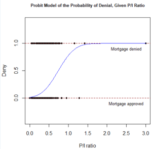
denyprobit <- glm(deny ~ pirat,
family = binomial(link = “probit”),
data = HMDA)
summary(denyprobit)
windows()
# plot data
plot(x = HMDA$pirat,
y = HMDA$deny,
main = “Probit Model of the Probability of Denial, Given P/I Ratio”,
xlab = “P/I ratio”,
ylab = “Deny”,
pch = 20,
ylim = c(-0.4, 1.4),
cex.main = 0.85)
# add horizontal dashed lines and text
abline(h = 1, lty = 2, col = “darkred”)
abline(h = 0, lty = 2, col = “darkred”)
text(2.5, 0.9, cex = 0.8, “Mortgage denied”)
text(2.5, -0.1, cex= 0.8, “Mortgage approved”)
# add estimated regression line
x <- seq(0, 3, 0.01)
y <- predict(denyprobit, list(pirat = x), type = “response”)
lines(x, y, lwd = 1.5, col = “blue”)
denyprobit2 <- glm(deny ~ pirat + black,
family = binomial(link = “probit”),
data = HMDA)
summary(denyprobit2)
library(stargazer)
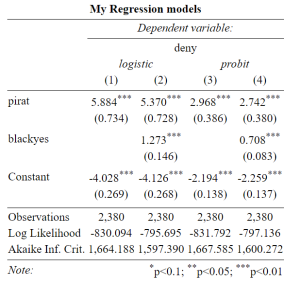
stargazer(denylogit,denylogit2,denyprobit,denyprobit2, type = “html”, out = “binary data analysis.html” ,title = “My Regression models”)
#修改這段試試
stargazer(denylogit,denylogit2,denyprobit,denyprobit2, type = “text“, out = “binary data analysis.text ” ,title = “My Regression models”)
windows()
# plot data
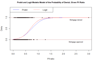
plot(x = HMDA$pirat,
y = HMDA$deny,
main = “Probit and Logit Models Model of the Probability of Denial, Given P/I Ratio”,
xlab = “P/I ratio”,
ylab = “Deny”,
pch = 20,
ylim = c(-0.4, 1.4),
cex.main = 0.9)
# add horizontal dashed lines and text
abline(h = 1, lty = 2, col = “darkred”)
abline(h = 0, lty = 2, col = “darkred”)
text(2.5, 0.9, cex = 0.8, “Mortgage denied”)
text(2.5, -0.1, cex= 0.8, “Mortgage approved”)
# add estimated regression line of Probit and Logit models
x <- seq(0, 3, 0.01)
y_probit <- predict(denyprobit, list(pirat = x), type = “response”)
y_logit <- predict(denylogit, list(pirat = x), type = “response”)
lines(x, y_probit, lwd = 1.5, col = “blue”)
#lines(x, y_logit, lwd = 1.5, col = “red”, lty = 2)
lines(x, y_logit, lwd = 1.5, col = “red”)
# add a legend
legend(“topleft”,
horiz = TRUE,
legend = c(“Probit”, “Logit”),
col = c(“blue”, “red”),
lty = c(1, 2))
